Inferential analyses

Last compiled on May, 2025

---

This is the code with which we run our inferential analyses.

---

1 Initatiating R environment

Start out with a custom function to load a set of required packages.

# packages and read data
rm(list = ls())

# (c) Jochem Tolsma
fpackage.check <- function(packages) {
    lapply(packages, FUN = function(x) {
        if (!require(x, character.only = TRUE)) {
            install.packages(x, dependencies = TRUE)
            library(x, character.only = TRUE)
        }
    })
}
packages = c("haven", "coda", "matrixStats", "parallel", "MASS", "doParallel", "dplyr", "cowplot", "tidyverse",
    "naniar", "dotwhisker", "gt", "reshape2", "VGAM", "expss", "Hmisc", "MASS", "sjPlot")
fpackage.check(packages)

#> [[1]]
#> NULL
#> 
#> [[2]]
#> NULL
#> 
#> [[3]]
#> NULL
#> 
#> [[4]]
#> NULL
#> 
#> [[5]]
#> NULL
#> 
#> [[6]]
#> NULL
#> 
#> [[7]]
#> NULL
#> 
#> [[8]]
#> NULL
#> 
#> [[9]]
#> NULL
#> 
#> [[10]]
#> NULL
#> 
#> [[11]]
#> NULL
#> 
#> [[12]]
#> NULL
#> 
#> [[13]]
#> NULL
#> 
#> [[14]]
#> NULL
#> 
#> [[15]]
#> NULL
#> 
#> [[16]]
#> NULL
#> 
#> [[17]]
#> NULL
#> 
#> [[18]]
#> NULL

rm(packages)
load("data/dutch_netsize_analyses_revision_2.rda")

---

2 Linear regression models

We run a series of regression models of logged acquantanceship network size (as it is right-skewed) on our independent and control variables. We thus run 172 different regression models (all scenarios).

# ######################## # MODELS ####################### # # age in categories, eval = false in
# 'independent_variables.rmd' fix later df$agecat[df$agecat == '18-30'] <- 1 df$agecat[df$agecat ==
# '31-45'] <- 2 df$agecat[df$agecat == '46-65'] <- 3 df$agecat[df$agecat == '>65'] <- 4
# table(df$agecat) class(df$agecat) # some final data handling to assign the correct reference
# categories df$opl <-relevel(df$opl, ref = 1) df$migr3 <-relevel(as.factor(df$migr3), ref = 1)
# df$income <-relevel(as.factor(df$income), ref = 2) df$agecat <-relevel(as.factor(df$agecat), ref
# = 4) # 172 regressions with different netsizes. We then look at distributions of coefficients
# across those.  # note the log10 for network size and how we don't take into account extreme
# network size.  modellog <- list() for (i in 14:185) { df[,c(i)] <- round(df[, c(i)], 0)
# modellog[[i]] <- lm(log10(df[!df[[i]]>5000, c(i)]) ~ as.factor(work) + hhsize + as.factor(migr3)
# + as.factor(agecat) + as.factor(income) + worthhouse + as.factor(woman) + as.factor(opl), data =
# df[!df[[i]]>5000,]) } modellog[sapply(modellog, is.null)] <- NULL summary(modellog[[1]])

---

3 Visualization of regression models

We then render all those models into one figure where we can show statistical signifance and that results do not vary over all those scenarios. This matches Figure 3 in the paper.

# #-------------------------------------------------------------------------------- # Viz of
# results # main effects four_brackets <- list( c('Dutch maj=ref', 'West backgr', 'non-West
# backgr'), c('>65=ref', '18-30', '46-65'), c('>modal inc=ref', '<=modal income', 'Unkn income'),
# c('Educ tert high=ref', 'Educ prim/sec', 'Educ tert low')) logmodel <- {dwplot(modellog, dot_args
# = list(color = 'black', size = 0.75, shape = 1), # color for the dot whisker_args = list(size =
# 0.25, color = 'darkgrey', alpha = 0.5), # color for the whisker vline =
# ggplot2::geom_vline(xintercept = 0, # put vline _behind_ coefs; see
# https://github.com/fsolt/dotwhisker/issues/84 colour = 'grey60', linetype = 2, linewidth = 1))
# %>% # make model variable relabel_predictors(c( 'as.factor(work)1' = 'Working', 'hhsize' =
# 'Household size', 'as.factor(migr3)2' = 'West backgr', 'as.factor(migr3)3' = 'non-West backgr',
# 'as.factor(agecat)1' = '18-30', 'as.factor(agecat)2' = '31-45', 'as.factor(agecat)3' = '46-65',
# 'as.factor(income)1' = '<=modal income', 'as.factor(income)3' = 'Unkn income', 'worthhouse' =
# 'House value', 'as.factor(woman)1' = 'Women', 'as.factor(opl)1' = 'Educ prim/sec',
# 'as.factor(opl)2' = 'Educ tert low' )) + theme(legend.position = 'none', axis.text =
# element_text(color = 'grey')) + theme_minimal() + xlab('B on Log(network size count)')} %>%
# add_brackets(four_brackets, fontSize = .6) ggsave('output/models.pdf', plot = logmodel, device =
# 'pdf', scale = 1, width = 6, height = 5, units = c('in'), dpi = 'retina') # Figure 3 in the paper
# logmodel

---

4 Regression table

We also average all 172 network size scenarios within respondents and run one single regression model so as to generate a table with coefficients. This matches Table 3 in the paper.

# df$netsize <- round(rowSums(df[,c(14:185)]) / length(14:185), 0) modell <- lm(log10(netsize) ~
# as.factor(work) + hhsize + as.factor(migr3) + as.factor(agecat) + as.factor(income) + worthhouse
# + as.factor(woman) + as.factor(opl), data = df[!df[['netsize']]>5000,]) modellin <- lm(netsize ~
# as.factor(work) + hhsize + as.factor(migr3) + as.factor(agecat) + as.factor(income) + worthhouse
# + as.factor(woman) + as.factor(opl), data = df[!df[['netsize']]>5000,]) fpackage.check('sjPlot')
# #table 3 in the paper tab_model(modell, modellin, show.se = TRUE)

# # robustness, migration two cats, and income no missings lead to similar results summary(x
# <-lm(log10(netsize) ~ as.factor(work) + hhsize + as.factor(migr) + as.factor(agecat) +
# as.factor(income) + worthhouse + as.factor(woman) + as.factor(opl), data =
# df[!df[['netsize']]>5000,])) summary(x <-lm(log10(netsize) ~ as.factor(work) + hhsize +
# as.factor(migr3) + as.factor(agecat) + as.factor(income) + worthhouse + as.factor(woman) +
# as.factor(opl), data = df[!df[['netsize']]>5000 & df$income != 3,]))

---

5 Revisions Regression table

From here onwards, we show our new results based on the revisions of this paper.

# # age in categories, eval = false in "independent_variables.rmd" fix later
df$agecat[df$agecat == "18-30"] <- 1
df$agecat[df$agecat == "31-45"] <- 2
df$agecat[df$agecat == "46-65"] <- 3
df$agecat[df$agecat == ">65"] <- 4

table(df$agecat)

#> 
#>   4   1   2   3 
#> 299 208 230 512

class(df$agecat)

#> [1] "factor"

# some final data handling to assign the correct reference categories
#df$opl2 <-relevel(as.factor(df$opl2), ref = 0)

df$agecat<- as.character(df$agecat)
df$income<- as.character(df$income)
df$income <-relevel(as.factor(df$income), ref = 2)
df$agecat <-relevel(as.factor(df$agecat), ref = 4)

table(df$opl2)

#> 
#>   0   1 
#> 783 466

summary(df$netsover1)

#>    Min. 1st Qu.  Median    Mean 3rd Qu.    Max. 
#>   18.23   95.43  146.04  166.94  208.88 1624.76

summary(df$netsover2)

#>    Min. 1st Qu.  Median    Mean 3rd Qu.    Max. 
#>   18.25   93.89  144.78  165.37  207.39 1604.70

summary(df$netsover3)

#>    Min. 1st Qu.  Median    Mean 3rd Qu.    Max. 
#>   248.9   438.4   997.9  1599.9  2216.2 27111.8

summary(df$netsover4)

#>    Min. 1st Qu.  Median    Mean 3rd Qu.    Max. 
#>   42.17  169.78  266.08  308.85  392.55 1991.33

summary(df$netsover5)

#>    Min. 1st Qu.  Median    Mean 3rd Qu.    Max. 
#>   15.80   84.18  129.69  149.67  187.15 1559.14

summary(df$netsover6)

#>    Min. 1st Qu.  Median    Mean 3rd Qu.    Max. 
#>    98.3   289.6   487.6   568.0   718.3  3590.9

DescTools::Desc(df$netsover6)

#> ────────────────────────────────────────────────────────────────────────────────────────────────── 
#> df$netsover6 (numeric)
#> 
#>        length          n        NAs     unique         0s         mean       meanCI'
#>         1'249      1'249          0        = n          0    568.04962    546.40874
#>                   100.0%       0.0%                  0.0%                 589.69050
#>                                                                                    
#>           .05        .10        .25     median        .75          .90          .95
#>     145.10962  189.16292  289.61668  487.56399  718.26326  1'036.32633  1'317.85350
#>                                                                                    
#>         range         sd      vcoef        mad        IQR         skew         kurt
#>   3'492.57384  389.84025    0.68628  304.19046  428.64658      2.03036      7.15149
#>                                                                                    
#> lowest : 98.29521, 98.78263, 98.94134, 100.64501, 102.14226
#> highest: 2'521.80046, 2'648.02827, 2'837.85118, 2'941.00644, 3'590.86905
#> 
#> ' 95%-CI (classic)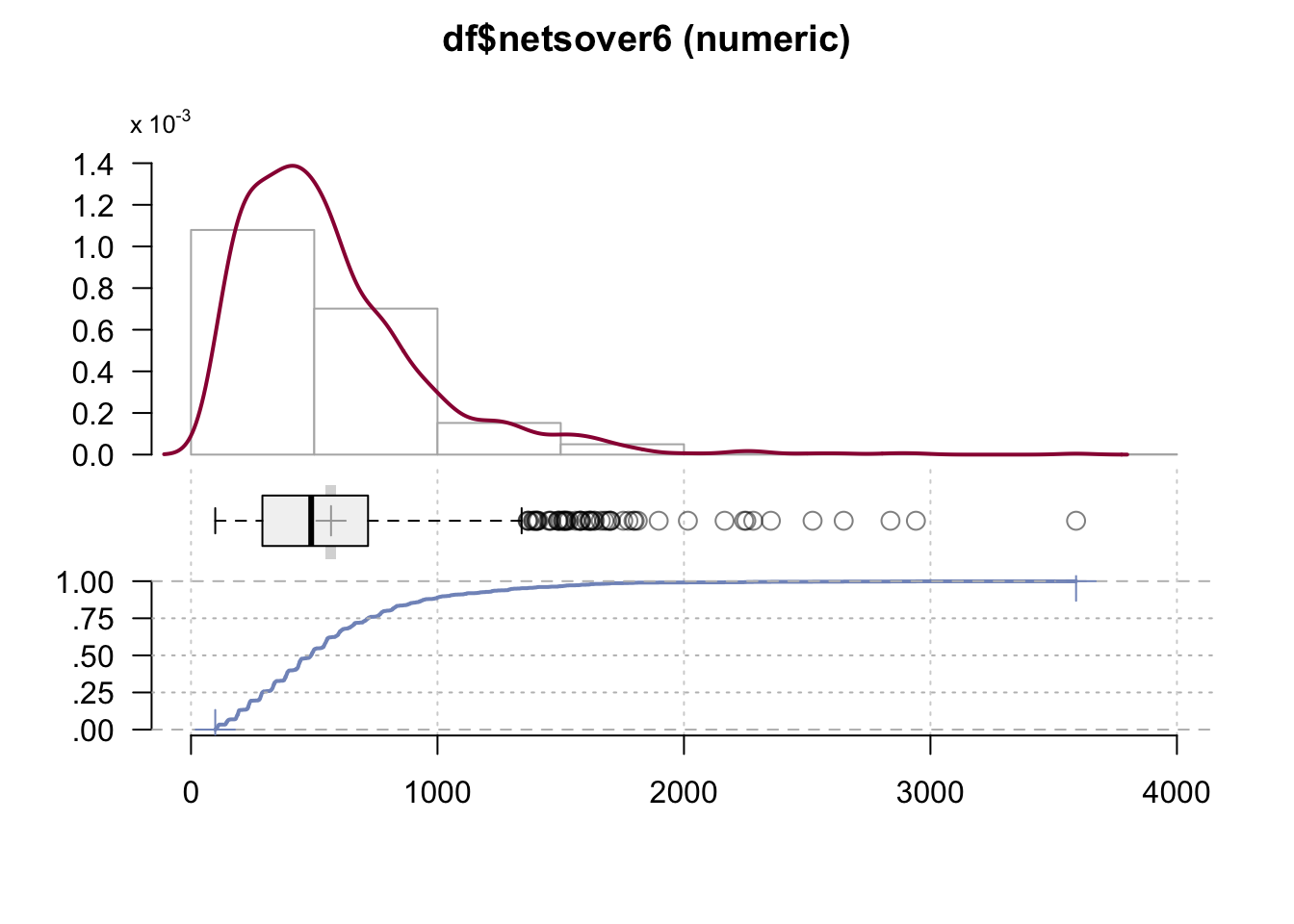

DescTools::Desc(df$netsover7)

#> ────────────────────────────────────────────────────────────────────────────────────────────────── 
#> df$netsover7 (numeric)
#> 
#>       length         n       NAs    unique        0s        mean      meanCI'
#>        1'249     1'249         0       = n         0    572.3718    550.4704
#>                 100.0%      0.0%                0.0%                594.2732
#>                                                                             
#>          .05       .10       .25    median       .75         .90         .95
#>     147.1833  192.0320  296.1159  495.6943  739.3279  1'043.0004  1'352.4317
#>                                                                             
#>        range        sd     vcoef       mad       IQR        skew        kurt
#>   3'574.6568  394.5333    0.6893  301.8440  443.2121      2.0620      7.4800
#>                                                                             
#> lowest : 94.8051, 100.1381, 101.2659, 101.3045, 101.516
#> highest: 2'537.0009, 2'676.8110, 2'829.6731, 3'086.7295, 3'669.4619
#> 
#> ' 95%-CI (classic)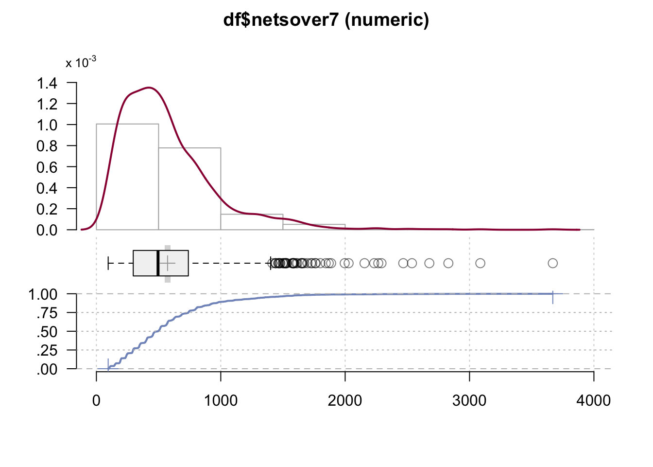

modell2 <- lm(log(netsover6) ~ 
                          as.factor(work) + #h1
                           
                          hhsize + #H2

                          as.factor(agecat) + #h3
                          
                          as.factor(income) + #h4
                          
                          worthhouse + #H4
                          
                          as.factor(woman) + #h5
                          
                          as.factor(opl2), #h6
                        data = df[!df[["netsover6"]]>2500,])
summary(modell2)

#> 
#> Call:
#> lm(formula = log(netsover6) ~ as.factor(work) + hhsize + as.factor(agecat) + 
#>     as.factor(income) + worthhouse + as.factor(woman) + as.factor(opl2), 
#>     data = df[!df[["netsover6"]] > 2500, ])
#> 
#> Residuals:
#>      Min       1Q   Median       3Q      Max 
#> -1.74525 -0.38338  0.02472  0.39268  1.63070 
#> 
#> Coefficients:
#>                    Estimate Std. Error t value Pr(>|t|)    
#> (Intercept)         5.61480    0.08040  69.834  < 2e-16 ***
#> as.factor(work)1    0.15854    0.04354   3.642 0.000282 ***
#> hhsize              0.08166    0.01647   4.957 8.17e-07 ***
#> as.factor(agecat)1  0.31600    0.06317   5.002 6.48e-07 ***
#> as.factor(agecat)2  0.16268    0.06493   2.505 0.012362 *  
#> as.factor(agecat)3  0.10123    0.05193   1.949 0.051479 .  
#> as.factor(income)1 -0.07853    0.04269  -1.839 0.066098 .  
#> as.factor(income)3 -0.07534    0.05669  -1.329 0.184063    
#> worthhouse          0.05362    0.02017   2.659 0.007941 ** 
#> as.factor(woman)1   0.01680    0.03524   0.477 0.633614    
#> as.factor(opl2)1    0.07790    0.03955   1.970 0.049100 *  
#> ---
#> Signif. codes:  0 '***' 0.001 '**' 0.01 '*' 0.05 '.' 0.1 ' ' 1
#> 
#> Residual standard error: 0.6057 on 1233 degrees of freedom
#> Multiple R-squared:  0.1232, Adjusted R-squared:  0.1161 
#> F-statistic: 17.32 on 10 and 1233 DF,  p-value: < 2.2e-16

modellnb2 <- glm.nb(netsover6 ~ 
                          as.factor(work) + 
                          
                          hhsize + 
                          
                          as.factor(agecat) + 
                          
                          as.factor(income) + 
                          
                          worthhouse +
                          
                          as.factor(woman) + 
                          
                          as.factor(opl2),
                        data = df[!df[["netsover6"]]>2500,],
                        init.theta = 1.032713156, link = log)
summary(modellnb2)

#> 
#> Call:
#> glm.nb(formula = netsover6 ~ as.factor(work) + hhsize + as.factor(agecat) + 
#>     as.factor(income) + worthhouse + as.factor(woman) + as.factor(opl2), 
#>     data = df[!df[["netsover6"]] > 2500, ], init.theta = 3.02530196, 
#>     link = log)
#> 
#> Coefficients:
#>                     Estimate Std. Error z value Pr(>|z|)    
#> (Intercept)         5.849823   0.076534  76.435  < 2e-16 ***
#> as.factor(work)1    0.127663   0.041442   3.080  0.00207 ** 
#> hhsize              0.070763   0.015676   4.514 6.36e-06 ***
#> as.factor(agecat)1  0.333836   0.060129   5.552 2.82e-08 ***
#> as.factor(agecat)2  0.175475   0.061822   2.838  0.00453 ** 
#> as.factor(agecat)3  0.106753   0.049456   2.159  0.03089 *  
#> as.factor(income)1 -0.069935   0.040639  -1.721  0.08527 .  
#> as.factor(income)3 -0.040986   0.053958  -0.760  0.44749    
#> worthhouse          0.044900   0.019192   2.340  0.01931 *  
#> as.factor(woman)1  -0.007934   0.033544  -0.237  0.81303    
#> as.factor(opl2)1    0.075745   0.037642   2.012  0.04419 *  
#> ---
#> Signif. codes:  0 '***' 0.001 '**' 0.01 '*' 0.05 '.' 0.1 ' ' 1
#> 
#> (Dispersion parameter for Negative Binomial(3.0253) family taken to be 1)
#> 
#>     Null deviance: 1473.5  on 1243  degrees of freedom
#> Residual deviance: 1311.0  on 1233  degrees of freedom
#> AIC: 17570
#> 
#> Number of Fisher Scoring iterations: 1
#> 
#> 
#>               Theta:  3.025 
#>           Std. Err.:  0.116 
#> 
#>  2 x log-likelihood:  -17546.061

fpackage.check("sjPlot")

#> [[1]]
#> NULL

# table 3 paper, (negbin is in appendix)
tab_model(modell2, modellnb2, show.se = TRUE)

	log(netsover6)				netsover6
Predictors	Estimates	std. Error	CI	p	Incidence Rate Ratios	std. Error	CI	p
(Intercept)	5.61	0.08	5.46 – 5.77	<0.001	347.17	26.57	298.37 – 404.03	<0.001
work [1]	0.16	0.04	0.07 – 0.24	<0.001	1.14	0.05	1.05 – 1.23	0.002
hhsize	0.08	0.02	0.05 – 0.11	<0.001	1.07	0.02	1.04 – 1.11	<0.001
agecat [1]	0.32	0.06	0.19 – 0.44	<0.001	1.40	0.08	1.24 – 1.57	<0.001
agecat [2]	0.16	0.06	0.04 – 0.29	0.012	1.19	0.07	1.06 – 1.34	0.005
agecat [3]	0.10	0.05	-0.00 – 0.20	0.051	1.11	0.06	1.01 – 1.23	0.031
income [1]	-0.08	0.04	-0.16 – 0.01	0.066	0.93	0.04	0.86 – 1.01	0.085
income [3]	-0.08	0.06	-0.19 – 0.04	0.184	0.96	0.05	0.86 – 1.07	0.447
worthhouse	0.05	0.02	0.01 – 0.09	0.008	1.05	0.02	1.01 – 1.09	0.019
woman [1]	0.02	0.04	-0.05 – 0.09	0.634	0.99	0.03	0.93 – 1.06	0.813
opl2 [1]	0.08	0.04	0.00 – 0.16	0.049	1.08	0.04	1.00 – 1.16	0.044
Observations	1244				1244
R2 / R2 adjusted	0.123 / 0.116				0.176

#gender

summary(df$perwomen)

#>    Min. 1st Qu.  Median    Mean 3rd Qu.    Max.    NA's 
#>  0.0000  0.4800  0.6571  0.6108  0.7861  1.0000      11

modelwoman <- lm(perwomen*100 ~ 
                          as.factor(work) +
                           
                          hhsize + 
                   
                          as.factor(agecat) + 
                          
                          as.factor(income) + 
                          
                          worthhouse + 
                          
                          as.factor(woman) + #h7
                          
                          as.factor(opl2), 
                        data = df)
summary(modelwoman)

#> 
#> Call:
#> lm(formula = perwomen * 100 ~ as.factor(work) + hhsize + as.factor(agecat) + 
#>     as.factor(income) + worthhouse + as.factor(woman) + as.factor(opl2), 
#>     data = df)
#> 
#> Residuals:
#>     Min      1Q  Median      3Q     Max 
#> -68.469 -13.189   4.078  16.113  46.832 
#> 
#> Coefficients:
#>                    Estimate Std. Error t value Pr(>|t|)    
#> (Intercept)         49.8266     3.0446  16.365  < 2e-16 ***
#> as.factor(work)1    -0.4459     1.6524  -0.270  0.78732    
#> hhsize               0.9540     0.6241   1.529  0.12661    
#> as.factor(agecat)1   2.3957     2.3898   1.002  0.31632    
#> as.factor(agecat)2   1.0720     2.4553   0.437  0.66248    
#> as.factor(agecat)3   1.6652     1.9756   0.843  0.39946    
#> as.factor(income)1   1.6213     1.6188   1.002  0.31677    
#> as.factor(income)3   1.9798     2.1508   0.921  0.35748    
#> worthhouse           0.3215     0.7626   0.422  0.67342    
#> as.factor(woman)1    9.0881     1.3365   6.800 1.63e-11 ***
#> as.factor(opl2)1     4.1546     1.5007   2.768  0.00572 ** 
#> ---
#> Signif. codes:  0 '***' 0.001 '**' 0.01 '*' 0.05 '.' 0.1 ' ' 1
#> 
#> Residual standard error: 22.91 on 1227 degrees of freedom
#>   (11 observations deleted due to missingness)
#> Multiple R-squared:  0.05174,    Adjusted R-squared:  0.04402 
#> F-statistic: 6.695 on 10 and 1227 DF,  p-value: 3.394e-10

modelman <- lm(permen*100 ~ 
                         as.factor(work) +
                           
                          hhsize + 
                   
                          as.factor(agecat) + 
                          
                          as.factor(income) + 
                          
                          worthhouse + 
                          
                          as.factor(woman) + #h7
                          
                          as.factor(opl2), 
                        data = df)
summary(modelman)

#> 
#> Call:
#> lm(formula = permen * 100 ~ as.factor(work) + hhsize + as.factor(agecat) + 
#>     as.factor(income) + worthhouse + as.factor(woman) + as.factor(opl2), 
#>     data = df)
#> 
#> Residuals:
#>     Min      1Q  Median      3Q     Max 
#> -46.832 -16.113  -4.078  13.189  68.469 
#> 
#> Coefficients:
#>                    Estimate Std. Error t value Pr(>|t|)    
#> (Intercept)         50.1734     3.0446  16.479  < 2e-16 ***
#> as.factor(work)1     0.4459     1.6524   0.270  0.78732    
#> hhsize              -0.9540     0.6241  -1.529  0.12661    
#> as.factor(agecat)1  -2.3957     2.3898  -1.002  0.31632    
#> as.factor(agecat)2  -1.0720     2.4553  -0.437  0.66248    
#> as.factor(agecat)3  -1.6652     1.9756  -0.843  0.39946    
#> as.factor(income)1  -1.6213     1.6188  -1.002  0.31677    
#> as.factor(income)3  -1.9798     2.1508  -0.921  0.35748    
#> worthhouse          -0.3215     0.7626  -0.422  0.67342    
#> as.factor(woman)1   -9.0881     1.3365  -6.800 1.63e-11 ***
#> as.factor(opl2)1    -4.1546     1.5007  -2.768  0.00572 ** 
#> ---
#> Signif. codes:  0 '***' 0.001 '**' 0.01 '*' 0.05 '.' 0.1 ' ' 1
#> 
#> Residual standard error: 22.91 on 1227 degrees of freedom
#>   (11 observations deleted due to missingness)
#> Multiple R-squared:  0.05174,    Adjusted R-squared:  0.04402 
#> F-statistic: 6.695 on 10 and 1227 DF,  p-value: 3.394e-10

summary(df$permen)

#>    Min. 1st Qu.  Median    Mean 3rd Qu.    Max.    NA's 
#>  0.0000  0.2139  0.3429  0.3892  0.5200  1.0000      11

summary(df$perwomen)

#>    Min. 1st Qu.  Median    Mean 3rd Qu.    Max.    NA's 
#>  0.0000  0.4800  0.6571  0.6108  0.7861  1.0000      11

modelsamegen <- lm(samegender*100 ~ 
                     
                         as.factor(work) +
                           
                          hhsize + 
                   
                          as.factor(agecat) + 
                          
                          as.factor(income) + 
                          
                          worthhouse + 
                          
                          as.factor(woman) + #h7
                          
                          as.factor(opl2), 
                        data = df)
summary(modelsamegen)

#> 
#> Call:
#> lm(formula = samegender * 100 ~ as.factor(work) + hhsize + as.factor(agecat) + 
#>     as.factor(income) + worthhouse + as.factor(woman) + as.factor(opl2), 
#>     data = df)
#> 
#> Residuals:
#>     Min      1Q  Median      3Q     Max 
#> -67.160 -14.994   1.213  15.343  59.364 
#> 
#> Coefficients:
#>                    Estimate Std. Error t value Pr(>|t|)    
#> (Intercept)        42.44446    3.05418  13.897   <2e-16 ***
#> as.factor(work)1    1.80866    1.65755   1.091    0.275    
#> hhsize              0.06058    0.62601   0.097    0.923    
#> as.factor(agecat)1  1.09655    2.39727   0.457    0.647    
#> as.factor(agecat)2  0.67618    2.46299   0.275    0.784    
#> as.factor(agecat)3  1.94900    1.98180   0.983    0.326    
#> as.factor(income)1 -1.51583    1.62388  -0.933    0.351    
#> as.factor(income)3 -1.03683    2.15749  -0.481    0.631    
#> worthhouse         -0.11878    0.76494  -0.155    0.877    
#> as.factor(woman)1  22.22627    1.34072  16.578   <2e-16 ***
#> as.factor(opl2)1    0.41080    1.50543   0.273    0.785    
#> ---
#> Signif. codes:  0 '***' 0.001 '**' 0.01 '*' 0.05 '.' 0.1 ' ' 1
#> 
#> Residual standard error: 22.98 on 1227 degrees of freedom
#>   (11 observations deleted due to missingness)
#> Multiple R-squared:  0.1903, Adjusted R-squared:  0.1837 
#> F-statistic: 28.83 on 10 and 1227 DF,  p-value: < 2.2e-16

tab_model(modelwoman, modelsamegen, show.se = TRUE)

	perwomen * 100				samegender * 100
Predictors	Estimates	std. Error	CI	p	Estimates	std. Error	CI	p
(Intercept)	49.83	3.04	43.85 – 55.80	<0.001	42.44	3.05	36.45 – 48.44	<0.001
work [1]	-0.45	1.65	-3.69 – 2.80	0.787	1.81	1.66	-1.44 – 5.06	0.275
hhsize	0.95	0.62	-0.27 – 2.18	0.127	0.06	0.63	-1.17 – 1.29	0.923
agecat [1]	2.40	2.39	-2.29 – 7.08	0.316	1.10	2.40	-3.61 – 5.80	0.647
agecat [2]	1.07	2.46	-3.75 – 5.89	0.662	0.68	2.46	-4.16 – 5.51	0.784
agecat [3]	1.67	1.98	-2.21 – 5.54	0.399	1.95	1.98	-1.94 – 5.84	0.326
income [1]	1.62	1.62	-1.55 – 4.80	0.317	-1.52	1.62	-4.70 – 1.67	0.351
income [3]	1.98	2.15	-2.24 – 6.20	0.357	-1.04	2.16	-5.27 – 3.20	0.631
worthhouse	0.32	0.76	-1.17 – 1.82	0.673	-0.12	0.76	-1.62 – 1.38	0.877
woman [1]	9.09	1.34	6.47 – 11.71	<0.001	22.23	1.34	19.60 – 24.86	<0.001
opl2 [1]	4.15	1.50	1.21 – 7.10	0.006	0.41	1.51	-2.54 – 3.36	0.785
Observations	1238				1238
R2 / R2 adjusted	0.052 / 0.044				0.190 / 0.184

# line educ independent variable up to educ homogeneity dependent
summary(df$pereduchigh)

#>    Min. 1st Qu.  Median    Mean 3rd Qu.    Max.    NA's 
#>   0.000   0.400   0.750   0.652   1.000   1.000     640

#educ
modeleduch <- lm(pereduchigh*100 ~ 
                          as.factor(work) +
                           
                          hhsize + 
                   
                          as.factor(agecat) + 
                          
                          as.factor(income) + 
                          
                          worthhouse + 
                          
                          as.factor(woman) + 
                          
                          as.factor(opl2), # h8
                        data = df)
summary(modeleduch)

#> 
#> Call:
#> lm(formula = pereduchigh * 100 ~ as.factor(work) + hhsize + as.factor(agecat) + 
#>     as.factor(income) + worthhouse + as.factor(woman) + as.factor(opl2), 
#>     data = df)
#> 
#> Residuals:
#>     Min      1Q  Median      3Q     Max 
#> -93.837 -19.409   6.789  22.336  58.169 
#> 
#> Coefficients:
#>                    Estimate Std. Error t value Pr(>|t|)    
#> (Intercept)         57.3799     6.5958   8.700  < 2e-16 ***
#> as.factor(work)1    -3.2362     3.3907  -0.954  0.34025    
#> hhsize              -3.7515     1.2737  -2.945  0.00335 ** 
#> as.factor(agecat)1   8.7501     4.9404   1.771  0.07705 .  
#> as.factor(agecat)2  -0.7916     5.5923  -0.142  0.88748    
#> as.factor(agecat)3  -5.5373     4.6698  -1.186  0.23619    
#> as.factor(income)1  -4.0102     3.3643  -1.192  0.23374    
#> as.factor(income)3  -4.6119     4.6984  -0.982  0.32670    
#> worthhouse           3.1077     1.5480   2.008  0.04514 *  
#> as.factor(woman)1    2.3365     2.8131   0.831  0.40656    
#> as.factor(opl2)1    24.7144     3.0722   8.045 4.67e-15 ***
#> ---
#> Signif. codes:  0 '***' 0.001 '**' 0.01 '*' 0.05 '.' 0.1 ' ' 1
#> 
#> Residual standard error: 33.87 on 598 degrees of freedom
#>   (640 observations deleted due to missingness)
#> Multiple R-squared:  0.1881, Adjusted R-squared:  0.1745 
#> F-statistic: 13.86 on 10 and 598 DF,  p-value: < 2.2e-16

modeleducl <- lm(pereduclow*100 ~ 
                          as.factor(work) +
                           
                          hhsize + 
                   
                          as.factor(agecat) + 
                          
                          as.factor(income) + 
                          
                          worthhouse + 
                          
                          as.factor(woman) + 
                          
                          as.factor(opl2), # h8
                        data = df)
summary(modeleducl)

#> 
#> Call:
#> lm(formula = pereduclow * 100 ~ as.factor(work) + hhsize + as.factor(agecat) + 
#>     as.factor(income) + worthhouse + as.factor(woman) + as.factor(opl2), 
#>     data = df)
#> 
#> Residuals:
#>     Min      1Q  Median      3Q     Max 
#> -58.169 -22.336  -6.789  19.409  93.837 
#> 
#> Coefficients:
#>                    Estimate Std. Error t value Pr(>|t|)    
#> (Intercept)         42.6201     6.5958   6.462 2.15e-10 ***
#> as.factor(work)1     3.2362     3.3907   0.954  0.34025    
#> hhsize               3.7515     1.2737   2.945  0.00335 ** 
#> as.factor(agecat)1  -8.7501     4.9404  -1.771  0.07705 .  
#> as.factor(agecat)2   0.7916     5.5923   0.142  0.88748    
#> as.factor(agecat)3   5.5373     4.6698   1.186  0.23619    
#> as.factor(income)1   4.0102     3.3643   1.192  0.23374    
#> as.factor(income)3   4.6119     4.6984   0.982  0.32670    
#> worthhouse          -3.1077     1.5480  -2.008  0.04514 *  
#> as.factor(woman)1   -2.3365     2.8131  -0.831  0.40656    
#> as.factor(opl2)1   -24.7144     3.0722  -8.045 4.67e-15 ***
#> ---
#> Signif. codes:  0 '***' 0.001 '**' 0.01 '*' 0.05 '.' 0.1 ' ' 1
#> 
#> Residual standard error: 33.87 on 598 degrees of freedom
#>   (640 observations deleted due to missingness)
#> Multiple R-squared:  0.1881, Adjusted R-squared:  0.1745 
#> F-statistic: 13.86 on 10 and 598 DF,  p-value: < 2.2e-16

modelsameeduc <- lm(sameeduc*100 ~ 
                          as.factor(work) +
                           
                          hhsize + 
                   
                          as.factor(agecat) + 
                          
                          as.factor(income) + 
                          
                          worthhouse + 
                          
                          as.factor(woman) + 
                          
                          as.factor(opl2), # h8
                        data = df)
summary(modelsameeduc)

#> 
#> Call:
#> lm(formula = sameeduc * 100 ~ as.factor(work) + hhsize + as.factor(agecat) + 
#>     as.factor(income) + worthhouse + as.factor(woman) + as.factor(opl2), 
#>     data = df)
#> 
#> Residuals:
#>     Min      1Q  Median      3Q     Max 
#> -89.997 -21.691   8.803  21.071  64.777 
#> 
#> Coefficients:
#>                    Estimate Std. Error t value Pr(>|t|)    
#> (Intercept)         34.6288     6.6859   5.179 3.05e-07 ***
#> as.factor(work)1     6.4881     3.4370   1.888   0.0595 .  
#> hhsize              -0.3228     1.2911  -0.250   0.8027    
#> as.factor(agecat)1   6.5634     5.0079   1.311   0.1905    
#> as.factor(agecat)2   7.3664     5.6687   1.299   0.1943    
#> as.factor(agecat)3   1.9065     4.7337   0.403   0.6873    
#> as.factor(income)1   1.4432     3.4102   0.423   0.6723    
#> as.factor(income)3  -3.5598     4.7626  -0.747   0.4551    
#> worthhouse           2.1065     1.5691   1.342   0.1800    
#> as.factor(woman)1    3.2038     2.8516   1.124   0.2617    
#> as.factor(opl2)1    30.0928     3.1142   9.663  < 2e-16 ***
#> ---
#> Signif. codes:  0 '***' 0.001 '**' 0.01 '*' 0.05 '.' 0.1 ' ' 1
#> 
#> Residual standard error: 34.34 on 598 degrees of freedom
#>   (640 observations deleted due to missingness)
#> Multiple R-squared:  0.2062, Adjusted R-squared:  0.193 
#> F-statistic: 15.54 on 10 and 598 DF,  p-value: < 2.2e-16

tab_model(modeleduch, modelsameeduc, show.se = TRUE)

	pereduchigh * 100				sameeduc * 100
Predictors	Estimates	std. Error	CI	p	Estimates	std. Error	CI	p
(Intercept)	57.38	6.60	44.43 – 70.33	<0.001	34.63	6.69	21.50 – 47.76	<0.001
work [1]	-3.24	3.39	-9.90 – 3.42	0.340	6.49	3.44	-0.26 – 13.24	0.060
hhsize	-3.75	1.27	-6.25 – -1.25	0.003	-0.32	1.29	-2.86 – 2.21	0.803
agecat [1]	8.75	4.94	-0.95 – 18.45	0.077	6.56	5.01	-3.27 – 16.40	0.190
agecat [2]	-0.79	5.59	-11.77 – 10.19	0.887	7.37	5.67	-3.77 – 18.50	0.194
agecat [3]	-5.54	4.67	-14.71 – 3.63	0.236	1.91	4.73	-7.39 – 11.20	0.687
income [1]	-4.01	3.36	-10.62 – 2.60	0.234	1.44	3.41	-5.25 – 8.14	0.672
income [3]	-4.61	4.70	-13.84 – 4.62	0.327	-3.56	4.76	-12.91 – 5.79	0.455
worthhouse	3.11	1.55	0.07 – 6.15	0.045	2.11	1.57	-0.98 – 5.19	0.180
woman [1]	2.34	2.81	-3.19 – 7.86	0.407	3.20	2.85	-2.40 – 8.80	0.262
opl2 [1]	24.71	3.07	18.68 – 30.75	<0.001	30.09	3.11	23.98 – 36.21	<0.001
Observations	609				609
R2 / R2 adjusted	0.188 / 0.175				0.206 / 0.193

Hypothesis 9: network size by homogeneity.

# genh9 <- lm(samegender ~ as.factor(work) + hhsize + as.factor(agecat) + as.factor(income) +
# worthhouse + as.factor(woman) + as.factor(opl2) + log(netsover4+1), #H9 data = df) educh9 <-
# lm(sameeduc ~ as.factor(work) + hhsize + as.factor(agecat) + as.factor(income) + worthhouse +
# as.factor(woman) + as.factor(opl2) + log(netsover4+1), #H9 data = df) summary(genh9)
# summary(educh9) tab_model(genh9, educh9, show.se = TRUE)

Ethnic background is dropped from the paper.

# #gender modeldutch <- lm(numdutch ~ as.factor(work) + hhsize + as.factor(migr3) +
# as.factor(agecat) + as.factor(income) + worthhouse + as.factor(woman) + as.factor(opl), data =
# df) #summary(modeldutch) modelnodutch <- lm(numnodutch ~ as.factor(work) + hhsize +
# as.factor(migr3) + as.factor(agecat) + as.factor(income) + worthhouse + as.factor(woman) +
# as.factor(opl), data = df) #summary(modelnodutch) modelsameethnic1 <- lm(sameethnic1 ~
# as.factor(work) + hhsize + as.factor(migr3) + as.factor(agecat) + as.factor(income) + worthhouse
# + as.factor(woman) + as.factor(opl), data = df) #summary(modelsameethnic1) tab_model(modeldutch,
# modelnodutch, modelsameethnic1, show.se = TRUE)

6 Revisions Robustness Regression table

# for each remove the top 5 highest points as outliers (though does not really matter)
DescTools::Desc(df$netsover1)

#> ────────────────────────────────────────────────────────────────────────────────────────────────── 
#> df$netsover1 (numeric)
#> 
#>        length          n       NAs     unique         0s       mean     meanCI'
#>         1'249      1'249         0        = n          0  166.93547  160.80197
#>                   100.0%      0.0%                  0.0%             173.06896
#>                                                                               
#>           .05        .10       .25     median        .75        .90        .95
#>      47.48610   62.21489  95.43336  146.04249  208.88463  293.42727  360.49569
#>                                                                               
#>         range         sd     vcoef        mad        IQR       skew       kurt
#>   1'606.52952  110.48917   0.66187   82.71617  113.45127    3.30686   28.45068
#>                                                                               
#> lowest : 18.22867, 19.06644, 19.23991, 19.37089, 19.39833
#> highest: 718.06718, 796.88416, 819.18232, 950.77244, 1'624.75819
#> 
#> ' 95%-CI (classic)

DescTools::Desc(df$netsover2)

#> ────────────────────────────────────────────────────────────────────────────────────────────────── 
#> df$netsover2 (numeric)
#> 
#>        length          n       NAs     unique         0s       mean     meanCI'
#>         1'249      1'249         0        = n          0  165.36984  159.29685
#>                   100.0%      0.0%                  0.0%             171.44282
#>                                                                               
#>           .05        .10       .25     median        .75        .90        .95
#>      47.11341   61.36250  93.89460  144.78071  207.39288  290.81353  356.98132
#>                                                                               
#>         range         sd     vcoef        mad        IQR       skew       kurt
#>   1'586.44801  109.39917   0.66154   82.04397  113.49828    3.29196   28.19860
#>                                                                               
#> lowest : 18.25379, 18.43516, 18.61252, 18.74904, 18.86651
#> highest: 705.75445, 789.28511, 808.8997, 946.3608, 1'604.70180
#> 
#> ' 95%-CI (classic)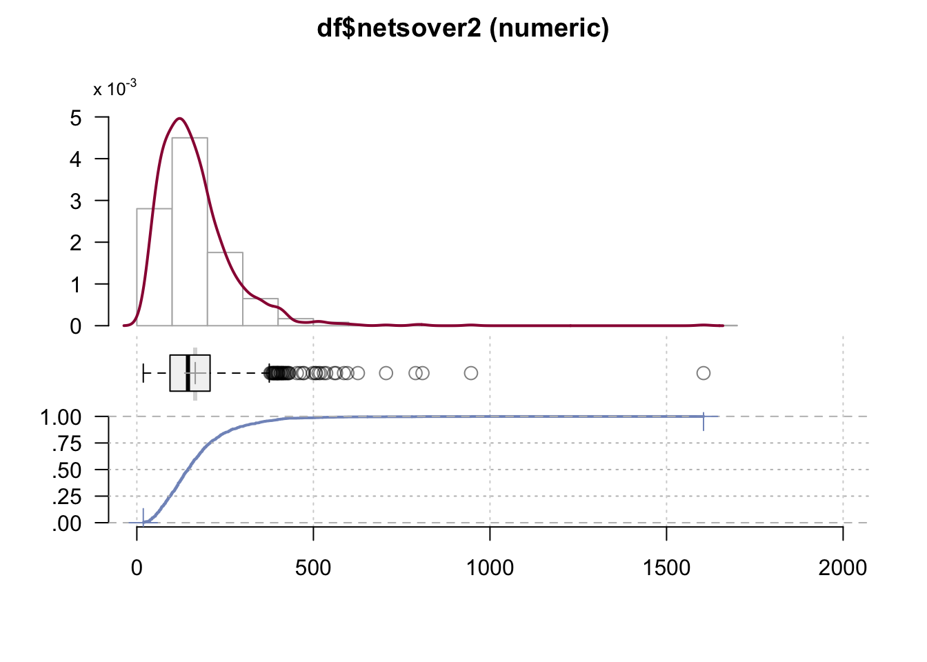

DescTools::Desc(df$netsover4)

#> ────────────────────────────────────────────────────────────────────────────────────────────────── 
#> df$netsover4 (numeric)
#> 
#>        length          n        NAs     unique         0s       mean     meanCI'
#>         1'249      1'249          0        = n          0  308.85362  297.06999
#>                   100.0%       0.0%                  0.0%             320.63725
#>                                                                                
#>           .05        .10        .25     median        .75        .90        .95
#>      72.70689  103.46361  169.77941  266.07913  392.54739  563.14906  711.50763
#>                                                                                
#>         range         sd      vcoef        mad        IQR       skew       kurt
#>   1'949.16115  212.27102    0.68729  163.56260  222.76798    2.21974    9.35343
#>                                                                                
#> lowest : 42.17049, 42.77368, 42.90526, 42.95338, 43.1082
#> highest: 1'409.49243, 1'431.57452, 1'740.46062, 1'862.98443, 1'991.33163
#> 
#> ' 95%-CI (classic)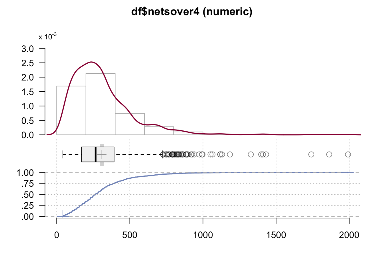

DescTools::Desc(df$netsover5)

#> ────────────────────────────────────────────────────────────────────────────────────────────────── 
#> df$netsover5 (numeric)
#> 
#>        length          n       NAs     unique         0s       mean     meanCI'
#>         1'249      1'249         0        = n          0  149.67066  144.00828
#>                   100.0%      0.0%                  0.0%             155.33305
#>                                                                               
#>           .05        .10       .25     median        .75        .90        .95
#>      40.72388   53.63708  84.17861  129.69246  187.15385  264.29139  326.98302
#>                                                                               
#>         range         sd     vcoef        mad        IQR       skew       kurt
#>   1'543.33313  102.00258   0.68151   74.94777  102.97524    3.56182   33.19883
#>                                                                               
#> lowest : 15.80333, 16.66687, 16.70652, 16.92885, 16.93847
#> highest: 653.82759, 708.11474, 777.8321, 859.73032, 1'559.13646
#> 
#> ' 95%-CI (classic)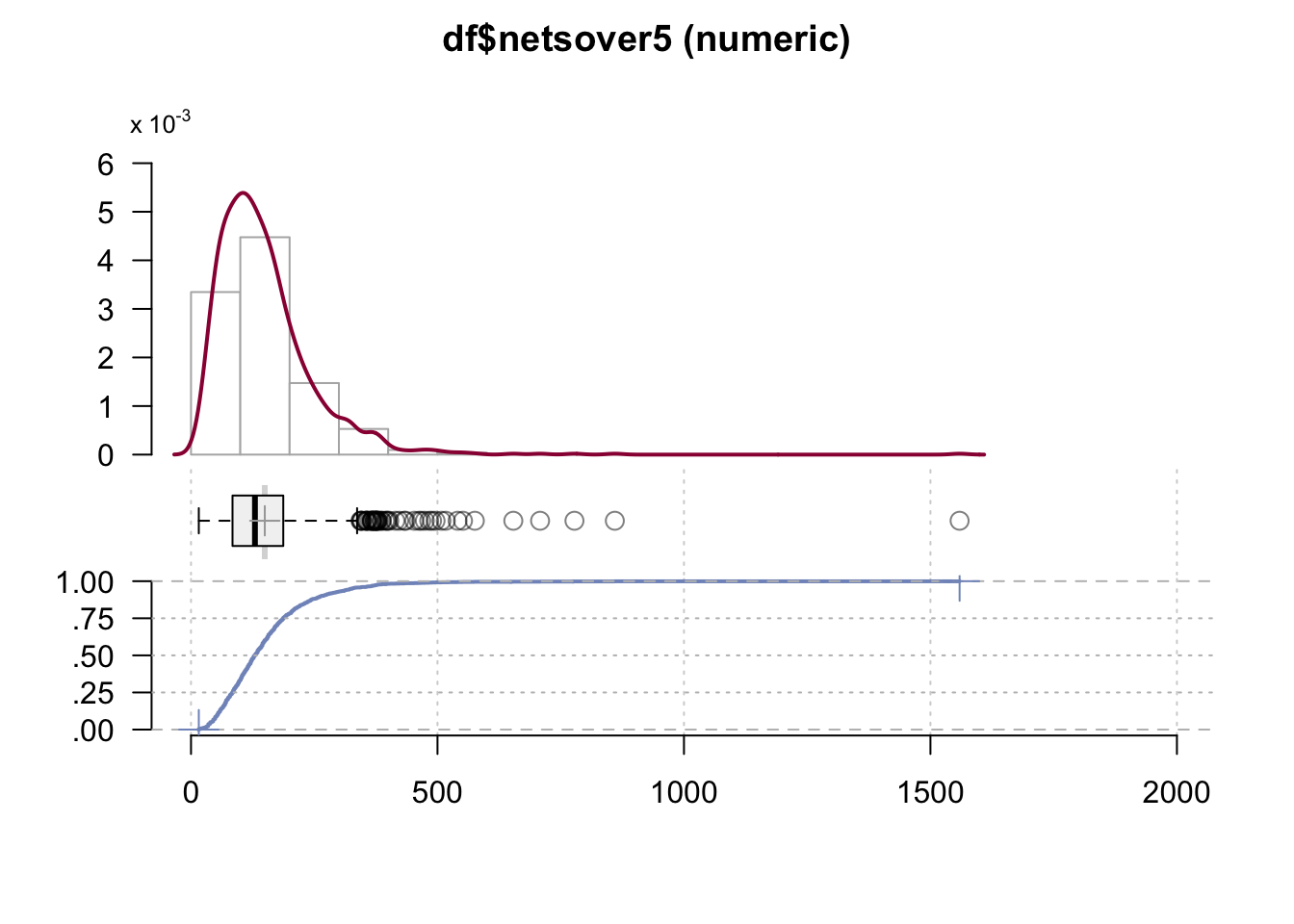

# robustness four other estimation scenarios: mostly qualitatively similar
r1 <- lm(log(netsover1) ~ 
                          as.factor(work) + #h1
                           
                          hhsize + #H2

                          as.factor(agecat) + #h3
                          
                          as.factor(income) + #h4
                          
                          worthhouse + #H4
                          
                          as.factor(woman) + #h5
                          
                          as.factor(opl2), #h6
                        data = df[!df[["netsover1"]]>700,])


r2 <- lm(log(netsover2) ~ 
                          as.factor(work) + #h1
                           
                          hhsize + #H2

                          as.factor(agecat) + #h3
                          
                          as.factor(income) + #h4
                          
                          worthhouse + #H4
                          
                          as.factor(woman) + #h5
                          
                          as.factor(opl2), #h6
                        data = df[!df[["netsover2"]]>700,])

r4 <- lm(log(netsover4) ~ 
                          as.factor(work) + #h1
                           
                          hhsize + #H2

                          as.factor(agecat) + #h3
                          
                          as.factor(income) + #h4
                          
                          worthhouse + #H4
                          
                          as.factor(woman) + #h5
                          
                          as.factor(opl2), #h6
                        data = df[!df[["netsover5"]]>1400,])


r5 <- lm(log(netsover5) ~ 
                          as.factor(work) + #h1
                           
                          hhsize + #H2

                          as.factor(agecat) + #h3
                          
                          as.factor(income) + #h4
                          
                          worthhouse + #H4
                          
                          as.factor(woman) + #h5
                          
                          as.factor(opl2), #h6
                        data = df[!df[["netsover5"]]>650,])

# robustness for scenarios
summary(r1)

#> 
#> Call:
#> lm(formula = log(netsover1) ~ as.factor(work) + hhsize + as.factor(agecat) + 
#>     as.factor(income) + worthhouse + as.factor(woman) + as.factor(opl2), 
#>     data = df[!df[["netsover1"]] > 700, ])
#> 
#> Residuals:
#>      Min       1Q   Median       3Q      Max 
#> -1.98276 -0.35765  0.01669  0.38832  1.58532 
#> 
#> Coefficients:
#>                     Estimate Std. Error t value Pr(>|t|)    
#> (Intercept)         4.571892   0.076643  59.652  < 2e-16 ***
#> as.factor(work)1    0.148253   0.041445   3.577 0.000361 ***
#> hhsize              0.070215   0.015722   4.466  8.7e-06 ***
#> as.factor(agecat)1  0.157371   0.060184   2.615 0.009036 ** 
#> as.factor(agecat)2  0.024436   0.061852   0.395 0.692863    
#> as.factor(agecat)3  0.038106   0.049487   0.770 0.441431    
#> as.factor(income)1 -0.095587   0.040737  -2.346 0.019110 *  
#> as.factor(income)3 -0.068747   0.053912  -1.275 0.202484    
#> worthhouse          0.036062   0.019213   1.877 0.060756 .  
#> as.factor(woman)1   0.008517   0.033606   0.253 0.799967    
#> as.factor(opl2)1    0.104288   0.037654   2.770 0.005696 ** 
#> ---
#> Signif. codes:  0 '***' 0.001 '**' 0.01 '*' 0.05 '.' 0.1 ' ' 1
#> 
#> Residual standard error: 0.5773 on 1233 degrees of freedom
#> Multiple R-squared:  0.0921, Adjusted R-squared:  0.08474 
#> F-statistic: 12.51 on 10 and 1233 DF,  p-value: < 2.2e-16

summary(r2)

#> 
#> Call:
#> lm(formula = log(netsover2) ~ as.factor(work) + hhsize + as.factor(agecat) + 
#>     as.factor(income) + worthhouse + as.factor(woman) + as.factor(opl2), 
#>     data = df[!df[["netsover2"]] > 700, ])
#> 
#> Residuals:
#>      Min       1Q   Median       3Q      Max 
#> -2.02275 -0.35692  0.01422  0.38906  1.59328 
#> 
#> Coefficients:
#>                     Estimate Std. Error t value Pr(>|t|)    
#> (Intercept)         4.560404   0.076771  59.403  < 2e-16 ***
#> as.factor(work)1    0.149088   0.041514   3.591 0.000342 ***
#> hhsize              0.070302   0.015748   4.464 8.78e-06 ***
#> as.factor(agecat)1  0.156478   0.060285   2.596 0.009553 ** 
#> as.factor(agecat)2  0.025234   0.061955   0.407 0.683857    
#> as.factor(agecat)3  0.036857   0.049569   0.744 0.457296    
#> as.factor(income)1 -0.095084   0.040804  -2.330 0.019954 *  
#> as.factor(income)3 -0.067367   0.054002  -1.247 0.212453    
#> worthhouse          0.036653   0.019245   1.905 0.057069 .  
#> as.factor(woman)1   0.008323   0.033662   0.247 0.804768    
#> as.factor(opl2)1    0.103671   0.037717   2.749 0.006071 ** 
#> ---
#> Signif. codes:  0 '***' 0.001 '**' 0.01 '*' 0.05 '.' 0.1 ' ' 1
#> 
#> Residual standard error: 0.5783 on 1233 degrees of freedom
#> Multiple R-squared:  0.09192,    Adjusted R-squared:  0.08456 
#> F-statistic: 12.48 on 10 and 1233 DF,  p-value: < 2.2e-16

summary(r4)

#> 
#> Call:
#> lm(formula = log(netsover4) ~ as.factor(work) + hhsize + as.factor(agecat) + 
#>     as.factor(income) + worthhouse + as.factor(woman) + as.factor(opl2), 
#>     data = df[!df[["netsover5"]] > 1400, ])
#> 
#> Residuals:
#>      Min       1Q   Median       3Q      Max 
#> -1.98182 -0.39475  0.04067  0.40970  2.37452 
#> 
#> Coefficients:
#>                    Estimate Std. Error t value Pr(>|t|)    
#> (Intercept)         5.01613    0.08271  60.648  < 2e-16 ***
#> as.factor(work)1    0.17128    0.04479   3.825 0.000138 ***
#> hhsize              0.07740    0.01698   4.558 5.67e-06 ***
#> as.factor(agecat)1  0.28426    0.06498   4.374 1.32e-05 ***
#> as.factor(agecat)2  0.15850    0.06678   2.374 0.017769 *  
#> as.factor(agecat)3  0.10696    0.05349   2.000 0.045767 *  
#> as.factor(income)1 -0.09177    0.04400  -2.086 0.037218 *  
#> as.factor(income)3 -0.10350    0.05831  -1.775 0.076155 .  
#> worthhouse          0.04865    0.02076   2.343 0.019266 *  
#> as.factor(woman)1   0.03149    0.03630   0.868 0.385770    
#> as.factor(opl2)1    0.11674    0.04071   2.867 0.004207 ** 
#> ---
#> Signif. codes:  0 '***' 0.001 '**' 0.01 '*' 0.05 '.' 0.1 ' ' 1
#> 
#> Residual standard error: 0.6246 on 1237 degrees of freedom
#> Multiple R-squared:  0.1235, Adjusted R-squared:  0.1165 
#> F-statistic: 17.44 on 10 and 1237 DF,  p-value: < 2.2e-16

summary(r5)

#> 
#> Call:
#> lm(formula = log(netsover5) ~ as.factor(work) + hhsize + as.factor(agecat) + 
#>     as.factor(income) + worthhouse + as.factor(woman) + as.factor(opl2), 
#>     data = df[!df[["netsover5"]] > 650, ])
#> 
#> Residuals:
#>      Min       1Q   Median       3Q      Max 
#> -2.22013 -0.37218  0.01684  0.39402  1.62133 
#> 
#> Coefficients:
#>                     Estimate Std. Error t value Pr(>|t|)    
#> (Intercept)         4.460242   0.078588  56.755  < 2e-16 ***
#> as.factor(work)1    0.148794   0.042496   3.501 0.000479 ***
#> hhsize              0.071489   0.016121   4.434 1.01e-05 ***
#> as.factor(agecat)1  0.142761   0.061711   2.313 0.020866 *  
#> as.factor(agecat)2  0.014148   0.063422   0.223 0.823508    
#> as.factor(agecat)3  0.026580   0.050743   0.524 0.600496    
#> as.factor(income)1 -0.097644   0.041770  -2.338 0.019566 *  
#> as.factor(income)3 -0.071227   0.055280  -1.288 0.197821    
#> worthhouse          0.036460   0.019700   1.851 0.064442 .  
#> as.factor(woman)1   0.007149   0.034459   0.207 0.835692    
#> as.factor(opl2)1    0.107697   0.038610   2.789 0.005362 ** 
#> ---
#> Signif. codes:  0 '***' 0.001 '**' 0.01 '*' 0.05 '.' 0.1 ' ' 1
#> 
#> Residual standard error: 0.592 on 1233 degrees of freedom
#> Multiple R-squared:  0.08768,    Adjusted R-squared:  0.08028 
#> F-statistic: 11.85 on 10 and 1233 DF,  p-value: < 2.2e-16

#gender
modelwoman <- lm(perwomen_red ~ 
                          as.factor(work) +
                           
                          hhsize + 
                   
                          as.factor(agecat) + 
                          
                          as.factor(income) + 
                          
                          worthhouse + 
                          
                          as.factor(woman) + #h7
                          
                          as.factor(opl2), 
                        data = df)
summary(modelwoman)

#> 
#> Call:
#> lm(formula = perwomen_red ~ as.factor(work) + hhsize + as.factor(agecat) + 
#>     as.factor(income) + worthhouse + as.factor(woman) + as.factor(opl2), 
#>     data = df)
#> 
#> Residuals:
#>     Min      1Q  Median      3Q     Max 
#> -0.6736 -0.1412  0.0431  0.1662  0.4958 
#> 
#> Coefficients:
#>                     Estimate Std. Error t value Pr(>|t|)    
#> (Intercept)         0.470454   0.030870  15.240  < 2e-16 ***
#> as.factor(work)1   -0.001346   0.016754  -0.080  0.93597    
#> hhsize              0.013783   0.006327   2.178  0.02957 *  
#> as.factor(agecat)1  0.004589   0.024231   0.189  0.84982    
#> as.factor(agecat)2 -0.008777   0.024895  -0.353  0.72448    
#> as.factor(agecat)3  0.007968   0.020031   0.398  0.69087    
#> as.factor(income)1  0.009504   0.016414   0.579  0.56269    
#> as.factor(income)3  0.026478   0.021807   1.214  0.22490    
#> worthhouse          0.006480   0.007732   0.838  0.40211    
#> as.factor(woman)1   0.092723   0.013551   6.842 1.23e-11 ***
#> as.factor(opl2)1    0.044743   0.015216   2.940  0.00334 ** 
#> ---
#> Signif. codes:  0 '***' 0.001 '**' 0.01 '*' 0.05 '.' 0.1 ' ' 1
#> 
#> Residual standard error: 0.2323 on 1227 degrees of freedom
#>   (11 observations deleted due to missingness)
#> Multiple R-squared:  0.05604,    Adjusted R-squared:  0.04835 
#> F-statistic: 7.285 on 10 and 1227 DF,  p-value: 2.846e-11

modelsamegen <- lm(samegender_red ~ 
                     
                         as.factor(work) +
                           
                          hhsize + 
                   
                          as.factor(agecat) + 
                          
                          as.factor(income) + 
                          
                          worthhouse + 
                          
                          as.factor(woman) + #h7
                          
                          as.factor(opl2), 
                        data = df)
summary(modelsamegen)

#> 
#> Call:
#> lm(formula = samegender_red ~ as.factor(work) + hhsize + as.factor(agecat) + 
#>     as.factor(income) + worthhouse + as.factor(woman) + as.factor(opl2), 
#>     data = df)
#> 
#> Residuals:
#>      Min       1Q   Median       3Q      Max 
#> -0.67160 -0.14994  0.01213  0.15343  0.59364 
#> 
#> Coefficients:
#>                      Estimate Std. Error t value Pr(>|t|)    
#> (Intercept)         0.4244446  0.0305418  13.897   <2e-16 ***
#> as.factor(work)1    0.0180866  0.0165755   1.091    0.275    
#> hhsize              0.0006058  0.0062601   0.097    0.923    
#> as.factor(agecat)1  0.0109655  0.0239727   0.457    0.647    
#> as.factor(agecat)2  0.0067618  0.0246299   0.275    0.784    
#> as.factor(agecat)3  0.0194900  0.0198180   0.983    0.326    
#> as.factor(income)1 -0.0151583  0.0162388  -0.933    0.351    
#> as.factor(income)3 -0.0103683  0.0215749  -0.481    0.631    
#> worthhouse         -0.0011878  0.0076494  -0.155    0.877    
#> as.factor(woman)1   0.2222627  0.0134072  16.578   <2e-16 ***
#> as.factor(opl2)1    0.0041080  0.0150543   0.273    0.785    
#> ---
#> Signif. codes:  0 '***' 0.001 '**' 0.01 '*' 0.05 '.' 0.1 ' ' 1
#> 
#> Residual standard error: 0.2298 on 1227 degrees of freedom
#>   (11 observations deleted due to missingness)
#> Multiple R-squared:  0.1903, Adjusted R-squared:  0.1837 
#> F-statistic: 28.83 on 10 and 1227 DF,  p-value: < 2.2e-16

#gender
modelwoman <- lm(perwomen_up ~ 
                          as.factor(work) +
                           
                          hhsize + 
                   
                          as.factor(agecat) + 
                          
                          as.factor(income) + 
                          
                          worthhouse + 
                          
                          as.factor(woman) + #h7
                          
                          as.factor(opl2), 
                        data = df)
summary(modelwoman)

#> 
#> Call:
#> lm(formula = perwomen_up ~ as.factor(work) + hhsize + as.factor(agecat) + 
#>     as.factor(income) + worthhouse + as.factor(woman) + as.factor(opl2), 
#>     data = df)
#> 
#> Residuals:
#>      Min       1Q   Median       3Q      Max 
#> -0.68486 -0.14204  0.04328  0.16784  0.49778 
#> 
#> Coefficients:
#>                     Estimate Std. Error t value Pr(>|t|)    
#> (Intercept)         0.465403   0.031205  14.915  < 2e-16 ***
#> as.factor(work)1   -0.001211   0.016935  -0.072  0.94298    
#> hhsize              0.013599   0.006396   2.126  0.03369 *  
#> as.factor(agecat)1  0.006779   0.024493   0.277  0.78200    
#> as.factor(agecat)2 -0.007160   0.025164  -0.285  0.77604    
#> as.factor(agecat)3  0.008147   0.020248   0.402  0.68750    
#> as.factor(income)1  0.008834   0.016591   0.532  0.59452    
#> as.factor(income)3  0.026769   0.022043   1.214  0.22483    
#> worthhouse          0.007169   0.007815   0.917  0.35915    
#> as.factor(woman)1   0.093073   0.013698   6.795 1.69e-11 ***
#> as.factor(opl2)1    0.045780   0.015381   2.976  0.00297 ** 
#> ---
#> Signif. codes:  0 '***' 0.001 '**' 0.01 '*' 0.05 '.' 0.1 ' ' 1
#> 
#> Residual standard error: 0.2348 on 1227 degrees of freedom
#>   (11 observations deleted due to missingness)
#> Multiple R-squared:  0.05599,    Adjusted R-squared:  0.04829 
#> F-statistic: 7.277 on 10 and 1227 DF,  p-value: 2.944e-11

modelsamegen <- lm(samegender_up ~ 
                     
                         as.factor(work) +
                           
                          hhsize + 
                   
                          as.factor(agecat) + 
                          
                          as.factor(income) + 
                          
                          worthhouse + 
                          
                          as.factor(woman) + #h7
                          
                          as.factor(opl2), 
                        data = df)
summary(modelsamegen)

#> 
#> Call:
#> lm(formula = samegender_up ~ as.factor(work) + hhsize + as.factor(agecat) + 
#>     as.factor(income) + worthhouse + as.factor(woman) + as.factor(opl2), 
#>     data = df)
#> 
#> Residuals:
#>      Min       1Q   Median       3Q      Max 
#> -0.65880 -0.15718  0.01288  0.16183  0.57276 
#> 
#> Coefficients:
#>                      Estimate Std. Error t value Pr(>|t|)    
#> (Intercept)         0.4515017  0.0313499  14.402   <2e-16 ***
#> as.factor(work)1    0.0162501  0.0170141   0.955    0.340    
#> hhsize             -0.0028425  0.0064258  -0.442    0.658    
#> as.factor(agecat)1  0.0074951  0.0246070   0.305    0.761    
#> as.factor(agecat)2  0.0230287  0.0252816   0.911    0.363    
#> as.factor(agecat)3  0.0221175  0.0203423   1.087    0.277    
#> as.factor(income)1 -0.0189660  0.0166685  -1.138    0.255    
#> as.factor(income)3 -0.0051859  0.0221457  -0.234    0.815    
#> worthhouse          0.0001680  0.0078518   0.021    0.983    
#> as.factor(woman)1   0.1789937  0.0137619  13.006   <2e-16 ***
#> as.factor(opl2)1    0.0007078  0.0154526   0.046    0.963    
#> ---
#> Signif. codes:  0 '***' 0.001 '**' 0.01 '*' 0.05 '.' 0.1 ' ' 1
#> 
#> Residual standard error: 0.2359 on 1227 degrees of freedom
#>   (11 observations deleted due to missingness)
#> Multiple R-squared:  0.1279, Adjusted R-squared:  0.1208 
#> F-statistic: 17.99 on 10 and 1227 DF,  p-value: < 2.2e-16